Justin Crites
Development
8
min read

Supabase announced their new Supabase Compute at their annual user conference, Supabase Select last week. Comput allows long-running services and agents to live inside your Supabase project, right next to the database itself. We were lucky enough to be invited into the private alpha so we quickly moved our Data Analyst Agent in for testing.
Answers came back 1.7× faster at 4.7× lower model cost. Access stayed read-only, and analysis still ran on snapshots, never on production. The more interesting part is why: once the data was a few milliseconds away instead of a few hundred, we could delete a lot of the machinery we’d built to work around the distance.
Here’s what Compute is, what we measured, and how it’s changing the way we build.
How our pipeline works today
Every Dreambase customer starts by connecting a Supabase project. From that moment, two rules shape everything our Data Analyst does:
The data stays on their Supabase: we don’t copy a customer’s database into our own infrastructure to analyze it.
Production gets as little exposure as possible: today, our agents don’t hold open connections to a customer’s production Postgres. They reach it through Supabase’s Management API, snapshot what they need, and do their analysis on that snapshot.
Those rules are why our pipeline looks the way it does: plan a dataset, snapshot it from the source, store it as Parquet, and answer questions from the stored dataset with DuckDB. It’s safe by design, but it means a lot of round trips between our servers and our customers’ databases.
That makes Compute an obvious fit: move the agent to the data instead of reaching across the internet for it. We tried it in two steps. First, we ran our existing pipeline on Compute; then we used what we learned to rethink the pipeline itself.
What Supabase Compute is
Supabase Compute is built for agentic workloads of two types:
Isolated sandboxes for running agent code
Always-on services
We used services. A service runs inside your Supabase project, on the same network as Postgres. You scaffold it with the Supabase CLI, push it, and Supabase builds and runs it.
Here are the basics during the alpha period. Details may change before general availability.
Runtimes. The
nodeanddenoruntimes deploy without a build step. Thedockerfileruntime builds any Dockerfile, and our small Deno service went live in about 3 seconds.Sizes. Instances come in
2gband4gb, with a configurable number of running copies.Exposure. A
publicservice gets an HTTPS endpoint athttps://<project-ref>.supabase.co/compute/v1/<service-name>. Aprivateservice has no URL and only makes outbound connections, which suits workers and queue consumers.Configuration. Project secrets arrive as environment variables, and running instances pick up changes within about a minute.
A service is a directory plus a few lines of config:
Why Compute and not Edge Functions
Supabase already runs code next to your database with Edge Functions, and in our latency tests below they came close: 4.3ms to Postgres, versus 2.9ms from Compute. The main difference is the type of the work you're doing. Edge Functions are built for request-bound tasks. Our agent is a Node server built from a Dockerfile that runs DuckDB and holds snapshots in memory across a multi-step run. A median complexity question takes ~18 seconds end-to-end.
Compute shines in this scenario because it gives that kind of process a full Linux environment with no limit on how long it runs.
Part 1: Our pipeline, moved onto Compute
Our Data Analyst is a custom-built harness on AI SDK that runs inside our own application on Vercel. For this experiment we ported it to eve, Vercel’s open-source, filesystem-first framework for durable backend AI agents. eve builds to a standard Node server, which we deployed with Docker.
We kept the pipeline’s four steps exactly as they are today:
Discover the connected schema.
Snapshot the data a question needs into an in-memory DuckDB dataset.
Answer from the snapshot with DuckDB, never from production.
Save the dataset to the customer’s Supabase Storage as Zstandard (zstd) compressed Parquet, so it can be reused later.
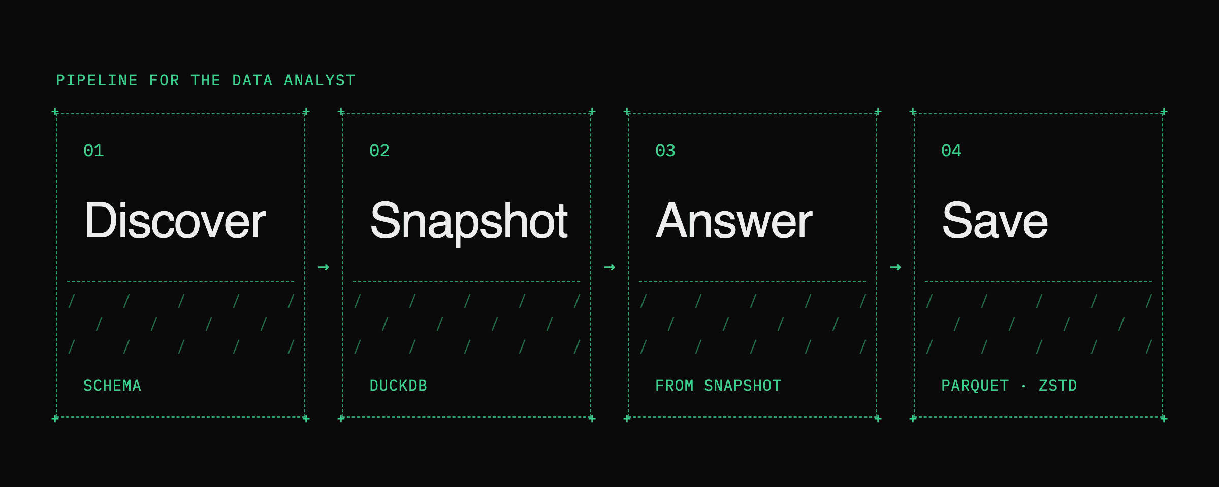
Every step now runs inside the customer’s Supabase project instead of reaching into it from outside. Two other things changed, and they matter for reading the results:
The path to the data. Instead of going through an API from our servers, the snapshot step connects to Postgres directly from inside the project, with a dedicated read-only role. Everything after the snapshot still runs on the snapshot, not on production.
The size of the agent. Running inside one customer’s project with one job to do, the agent carries only the four tools these steps need, not our full product toolkit.
The results
Compared with our current pipeline, the Compute version delivered:
1.7× faster answers: a median of 18.0s instead of 30.9s per question
4.7× lower model cost: $0.053 instead of $0.248 per question
11× fewer input tokens per question
18× faster dataset saves: 0.19s instead of 3.45s per question

Here's the full breakdown of what we were comparing:
Current pipeline | Pipeline on Compute | Improvement | |
|---|---|---|---|
Median time to answer | 30.9s | 18.0s | 1.7× faster |
90th-percentile time | 56.3s | 30.0s | 1.9× faster |
Model cost per question | $0.248 | $0.053 | 4.7× lower |
Model cost per 10,000 questions | $2,479 | $528 | $1,951 saved |
Input tokens per question | 253,461 | 23,550 | 11× fewer |
Model steps per question | 7.5 | 5.6 | 25% fewer |
Time saving the dataset | 3.45s | 0.19s | 18× faster |
When we benchmark, we aim to root them in real world scenarios that our customers deal with every day. Here's a few of the questions we used along with the performance of each, sorted by time saved:
Question | Current pipeline | On Compute | Time saved |
|---|---|---|---|
When did AI Insights launch, and how has adoption grown? | 64.0s | 23.3s | 40.7s |
Which 10 customers were most active in the last 30 days? | 37.8s | 16.9s | 20.9s |
Weekly active users for the last 8 complete weeks | 25.4s | 12.6s | 12.8s |
What changed with our Starter plan in early 2026? | 50.0s | 37.3s | 12.7s |
Weekday vs. weekend activity over the last 90 days | 27.1s | 16.5s | 10.6s |
Revenue collected each month in 2026 | 26.2s | 16.6s | 9.6s |
Paying customers and current MRR | 25.8s | 17.6s | 8.2s |
Trial-to-paid conversion by acquisition channel | 29.0s | 21.5s | 7.5s |
Where the time and money went
The 12.9 seconds saved on a median question come from two places.
Waiting for data - fell from 4.7s to 0.9s per question
Waiting for models - fell from 24.5s to 16.5s
With compute, we're able to focus the data analyst agent taking less steps with smaller prompts. The majority of the cost savings are driven from 11x fewer input tokens.
A lot of the cost savings for Dreambase stem from being able to slim our agent and shed some of the planning and coordination we built before every read became a few milliseconds away with Compute.
Single-digit milliseconds
Supabase says services on Compute reach Postgres in single-digit milliseconds. To check, we ran the same 14 analytics queries 10 times each from several places and timed only the query:

Path | Median per query |
|---|---|
Supabase Compute → Postgres, same region | 2.9ms |
Supabase Edge Function → Postgres, same region | 4.3ms |
A different region → Postgres, direct connection | 65ms |
Our current API-based query path, from a different region | 637ms |
A pipeline makes many of these calls per question, so taking each one from hundreds of milliseconds down to a few adds up quickly. It also says something about security. A direct connection from another region is 10× faster than our API path, but it would mean our servers holding a connection to a customer’s production database. Compute gets us better than direct-connection speed with the connection starting inside the customer’s own project. Less risk.
Snapshots isolate production from rogue agent queries
Snapshots are how we keep agent traffic off a customer’s production database, and on Compute they’re nearly free. Snapshotting all 419,158 product events into memory took about 1 second and 65MB. We then ran five analytics queries over the events table, once against live Postgres and once against the snapshot:
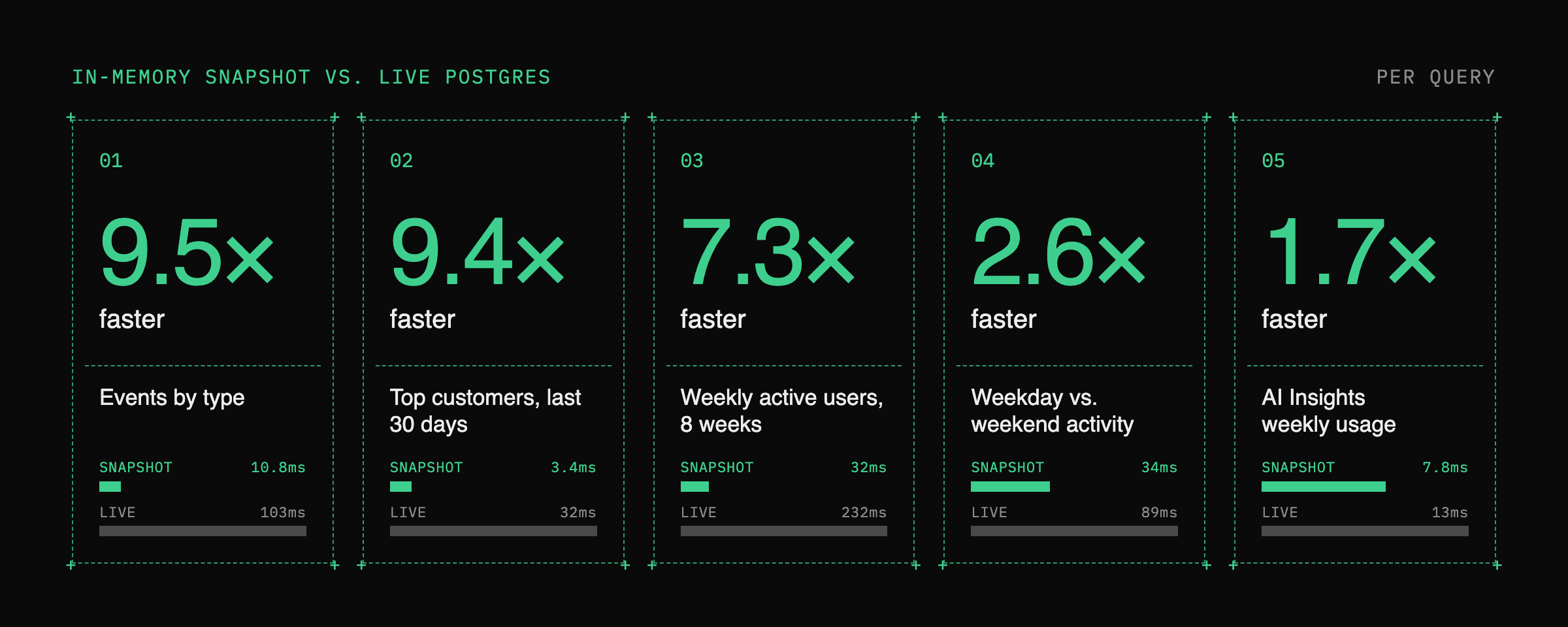
Query | Live Postgres | In-memory snapshot |
|---|---|---|
Events by type | 103ms | 10.8ms |
Top customers, last 30 days | 32ms | 3.4ms |
Weekly active users, 8 weeks | 232ms | 32ms |
Weekday vs. weekend activity | 189ms | 34ms |
AI Insights weekly usage | 13ms | 7.8ms |
After that one read, every query ran without touching production, and each finished 1.7–9.5× faster than the same query against live Postgres.
Part 2: Rethinking the pipeline
The early results made us step back and analyze how we’d built the pipeline in the first place. On Supabase Compute, the data is a few milliseconds away, so the database isn’t the slow part anymore. All the planning we built to work around the distance is now moot. That lets us flip the script, so the agent explores first and builds the dataset after. We’ve been calling these just-in-time datasets (we need marketing help). The agent queries a read-only copy of the customer’s data directly, digs around until it finds what it needs, and snapshots only the data its answer depends on. It works the same way across all our integrations, not just Supabase.
We prototyped it against the primary database with a dedicated read-only role. In production, that copy would be a read replica, so agent queries never land on the primary. The agent explores with read-only SQL, then saves one Parquet snapshot of the dataset behind its answer:
Current pipeline | Just-in-time Datasets | Improvement | |
|---|---|---|---|
Median time to answer | 30.9s | 16.4s | 1.9× faster |
Model cost per question | $0.248 | $0.051 | 4.9× lower |
Input tokens per question | 253,461 | 18,870 | 13× fewer |
Most of the savings come from what the agent no longer needs. With just-in-time datasets, it works from three focused tools instead of our full product toolkit. Fewer steps, and a much smaller prompt for each.
In an earlier run of the same benchmark, we also tried skipping the dataset save entirely. Against that run’s own baseline, the agent answered 2.3× faster at 6.2× lower cost, so there’s even more speed on the table when we don’t need to persist a dataset at all.
Nothing leaves the customer’s Supabase project except what the agent needs to answer the question at hand.
What we learned
If you’re building agents on Supabase, here’s what we’d take from this:
Latency in agent loops compounds: an app makes a handful of queries per page. With multiple queries (an agent makes many per question), 637ms vs 2.9ms per call really adds up.
Proximity lets you shrink the agent: most data agent scaffolding exists to work around slow data. Put the agent next to the data and you can cut it, saving tokens and cost, not just latency.
Snapshots keep agents off production for almost nothing: pulling 419,158 rows into in-memory DuckDB took about a second and 65MB. Every query after that ran without touching production. For more on why that matters, see our guide to giving an agent safe access to operational data.
Storage can be your dataset layer: zstd-compressed Parquet in Supabase Storage, read by DuckDB with range requests, means a query pulls only what it needs. More on that below.
What’s next: Storage as the dataset layer
Our datasets are already zstd-compressed Parquet, and our agents query them with DuckDB. Supabase Storage supports HTTP range requests, so DuckDB can read just the columns and row groups a query needs instead of downloading entire files. In our tests, a typical query read between 3% and 23% of a 5.4MB Parquet file.
That puts the whole loop inside the customer’s project:
Postgres and its read replicas for live data
Storage for saved datasets
Compute for the agent that works across both
Compute is still in private alpha, so (even though we really want) none of this on production (yet). We’re excited to keep building with the Supabase team as Compute moves toward general availability, and we’ll be rolling what we learned into Dreambase ASAP.
Thank you to Matt Johnston, Lakshan Perera, and the Supabase team for inviting us into the private alpha and for lightning fast answers to our questions.
Want to run your own agents next to your data? Supabase Compute is in private alpha.
By Justin Crites, Builder at Dreambase
Nitty gritty details on how we tested & measured
We built a database that mirrors a typical Dreambase customer: a B2B SaaS product with 1,500 companies, 6,825 users, subscriptions, invoices, support tickets, and 419,158 product events. It ran on a Supabase Micro instance, and our Compute services ran in the same region.
Eight analytics questions a founder or operator would actually ask, from “What’s our MRR?” to open-ended ones like “Something happened with our Starter plan in early 2026. What changed?”
Each question ran five times against each setup, in shuffled order, with a fresh session every time. Our current pipeline started from an empty workspace on every run, so no question benefited from a dataset saved earlier. Every setup saved a dataset as part of each answer, except the save-skipped oracle run described in Part 2. Compute instances were warm: the first call on a fresh instance adds several seconds of one-time setup.
Every run used Claude Opus 5.5 through Vercel AI Gateway, and costs come from the Gateway’s billing records for each model call.
FAQ
What is Supabase Compute?
Supabase Compute runs agent sandboxes and long-lived services inside a Supabase project, on the same network as its database and storage. Services use the node, deno, or dockerfile runtime, run on 2gb or 4gb instances, and are either public over HTTPS or private for background work. It was announced at Supabase Select 2026 and is currently in private alpha.
How is Supabase Compute different from Edge Functions?
Edge Functions are built for request-bound work. Compute services run as long as the work takes, in a full Linux environment, which suits agents, pipelines, and background jobs. In our tests, Compute reached Postgres in a median of 2.9ms, versus 4.3ms from an Edge Function in the same region.
How do I get access to Supabase Compute?
Join the waitlist on the Supabase Compute page. Supabase is rolling out invites during the private alpha.
Did running on Compute change Dreambase’s security model?
The safeguards stayed the same: access is read-only, analysis runs on snapshots rather than on production, and datasets are saved to the customer’s own Supabase Storage. What changed is the path to the data. Instead of reaching in through an API from our servers, the snapshot step connects from inside the customer’s project with a dedicated read-only role.
Why is the pipeline faster on Compute?
Two reasons. Our pipeline makes many small calls to the customer’s database for each question, and from Compute a query to Postgres in the same region took a median of 2.9ms, compared with 637ms through our current API path from a different region. And a focused agent next to the data takes fewer model steps with a much smaller prompt.
Where do the cost savings come from?
Most model cost comes from the context sent on every step. Running a focused agent next to the data cut input tokens per question by 11× for our existing pipeline and by 13× for the data oracle design. That lowered model cost per question from $0.248 to $0.053 and $0.051.
What is a data oracle?
It’s an agent that works directly over a read-only copy of a customer’s data, such as a read replica, explores what it needs, and snapshots only the dataset behind its answer. In our benchmark, it answered 1.9× faster than our current pipeline at 4.9× lower model cost.
Which model did you use?
Every benchmark run used Claude Opus 5.5 through Vercel AI Gateway. Costs come from the Gateway’s billing records for each model call.
What do you want to know from your data?
Get the answer now.